How to Play With LLMs
At their core, LLMs are just a high-order Markov model of language with a large number of parameters. All of their functionality – even stuff like finetuning and RLHF – can be represented and understood through this lens.
\[P_{\theta}(x_{i+1} | x_1, x_2, \dots, x_{i-1}) \tag{1}\]Where \(\theta\) are the many parameters of the LLM, \(x_i\) are a sequence of tokens representing some text.
This tutorial will walk through loading the Falcon-7b model from HuggingFace, show how to fine-tune it, and finally create some visualizations of the hidden representations inside the LLM.
Sourcing Compute
The GPU market is insane. I’ve rented GPU time on a few services like Google Colab, Google Compute Engine, and Paperspace. Overall, I think most services where you can get root access to your own Linux machine with an Nvidia GPU are fine.
Working on an mps (Apple Silicon) machine is sometimes limiting since there’s
a bit of development lag between advances in the field and creating a version
that runs on Apple Silicon.
Plus, the upper bound on GPU power is low compared to Nvidia, especially
multi-GPU stuff.
Colab is also limiting because you’re forced to use the GPU through an IPython kernel, which limits the amount of control you have. Google also tends to rug-pull long compute jobs, and you’re limited to 1 A100 and a notebook interface (unless you break Google’s rules against setting up an ssh tunnel, which could get you banned from Colab in the future).
Overall, you end up saving a lot of time by developing on the same (or at least similar) infrastructure as you plan to deploy in. I would recommend a Ubuntu server with a big GPU (I’m using one of Paperspace’s A100 instances with ML in a box). This guide should also work if you are on Apple Silicon with enough RAM to support Falcon-7b.
Environment Setup
I use Python virtual environments with the venv module
(docs) to keep my projects’
dependencies from influencing each other.
If you plan to deploy your code on a more diverse range of machines, consider
using a Docker or Singularity container as well.
>>> python3 -m venv venv       # make the virtual environment called "venv"
>>> source venv/bin/activate   # enable the environment
(venv)>>>
Once activated, install the requirements in requirements.txt:
numpy
matplotlib
pandas
jupyter
torch

# Transformer-related modules
transformers  		# huggingface transformers

einops
accelerate
xformers
(venv)>>> pip3 install -r requirements.txtLoading the Model
Thanks to the great work at HuggingFace, it’s very straight forward to load models and start playing with them.
from transformers import AutoTokenizer, AutoModelForCausalLM
import torch
import numpy

model_name = "tiiuae/falcon-7b"
print("Loading the tokenizer and model weights...")
tokenizer = AutoTokenizer.from_pretrained(model_name)
model = AutoModelForCausalLM.from_pretrained(model_name)
print("Done!")

# Use the model...
With this, Huggingface will download the weights to ~/.cache/huggingface and
load the model and its tokenizer for further use. It will take a while to
download the weights when you first run it.
Before we use the model, let’s take a look at some of its attributes:
# Take a look at the model:
print("The type of `model` is: ", type(model))
print("The type of `tokenizer` is: ", type(tokenizer))
print(f"\n`model` is currently on device `{model.device}`")
print(f"Number of parameters: ", model.num_parameters())
The output here should be:
The type of `model` is:  <class 'transformers.models.falcon.modeling_falcon.FalconForCausalLM'>
The type of `tokenizer` is:  <class 'transformers.tokenization_utils_fast.PreTrainedTokenizerFast'>

`model` is currently on device `cuda:0`
Number of parameters:  6921720704
As expected, this model has ~7 billion parameters. We can also take a look at
the architecture by printing the model object:
FalconForCausalLM(
  (transformer): FalconModel(
    (word_embeddings): Embedding(65024, 4544)
    (h): ModuleList(
      (0-31): 32 x FalconDecoderLayer(
        (self_attention): FalconAttention(
          (rotary_emb): FalconRotaryEmbedding()
          (query_key_value): FalconLinear(in_features=4544, out_features=4672, bias=False)
          (dense): FalconLinear(in_features=4544, out_features=4544, bias=False)
          (attention_dropout): Dropout(p=0.0, inplace=False)
        )
        (mlp): FalconMLP(
          (dense_h_to_4h): FalconLinear(in_features=4544, out_features=18176, bias=False)
          (act): GELU(approximate='none')
          (dense_4h_to_h): FalconLinear(in_features=18176, out_features=4544, bias=False)
        )
        (input_layernorm): LayerNorm((4544,), eps=1e-05, elementwise_affine=True)
      )
    )
    (ln_f): LayerNorm((4544,), eps=1e-05, elementwise_affine=True)
  )
  (lm_head): Linear(in_features=4544, out_features=65024, bias=False)
)
Using the Model
We are nearly ready to start using the model as a Markov chain – it’s most fundamental mathematical form! First, we send the model to the GPU so it can run fast:
# %% Move to the GPU
# check if cuda is available:
if torch.cuda.is_available():
    device = torch.device("cuda")
    print("There are %d GPU(s) available." % torch.cuda.device_count())
    print("We will use the GPU:", torch.cuda.get_device_name(0))
# check if mps is available
elif torch.backends.mps.is_available():
    device = torch.device("mps")
    print("We will use the MPS GPU:", device)

model = model.to(device)
model.eval() # get the model ready for inference
Let’s apply the LLM’s Markov model \(P_{\theta}\) to the sentence, “I love France. The capital of France is "”. In reality the LLM computes Equation 1 for all \(i = 1, \dots, N\) during the forward pass on tokens \(\{x_i\}_{i=1}^N\).
Tokenization
The first step is to tokenize our input string. Check out the OpenAI tokenizer demo for more information about BPE tokenization:
# %% Define the input text, convert it into tokens.
input_text = "I love France. The capital of France is \""
input_ids = tokenizer.encode(input_text, return_tensors="pt").to(device)
print("input_text: ", input_text)
print("input_ids: ", input_ids)
print("input_ids.shape: ", input_ids.shape)

# sanity check: let's decode the input_ids back into text
print("input_ids decoded: ", tokenizer.decode(input_ids[0]))
From which we get
input_text:  I love France. The capital of France is "
input_ids:  tensor([[  52, 1163, 5582,   25,  390, 4236,  275, 5582,  304,  204,   13]],
       device='cuda:0')
input_ids.shape:  torch.Size([1, 11])
input_ids decoded:  I love France. The capital of France is "
input_ids has a shape [batch, num_tokens] ([1, 11] in this case).
Inference
As mentioned above, a forward pass of the transformer results in next token prediction on ALL \(x_{i+1}\) for \(i = 1, \dots, N\). Let’s take a look for ourselves.
# %% Run inference on the tokenized input text.
output = model(input_ids)
print("Output object keys: ", output.keys())
print("Output logits shape: ", output.logits.shape)
The output object’s keys look like this:
Output object keys:  odict_keys(['logits', 'past_key_values'])
Output logits shape:  torch.Size([1, 11, 65024])
The past_key_values are generally used to cache representations that would
otherwise be recomputed during iterative generation.
The logits contain the next token prediction information we’re currently
interested in:
Here the shape [1, 11, 65024] corresponds to [batch, sequence_len,
vocabulary_size].
The sequence length is the same as the number of input tokens, and the
vocabulary_size is the total number of unique tokens in the model’s
vocabulary.
The logits from the model output are unnormalized – i.e., they don’t sum to 1.
Let’s apply a softmax() to get normalized probabilities for each token.
# %% Softmax the logits to get probabilities
# index the 0th logit batch (we have batch=1)
probs = torch.nn.functional.softmax(output['logits'][0], dim=-1)
probs = probs.cpu().detach().numpy()  # move to the cpu, convert to numpy array
probs.shape # [sequence_len, vocab_size]

# get the probabilities of the next token
next_token_probs = probs[-1,:]
Let’s have a look at the probability distribution over next tokens after the input string.
# %% Plot the probability distribution over the final token
import matplotlib.pyplot as plt
plt.plot(next_token_probs)
plt.title("Probability distribution over Final Token")
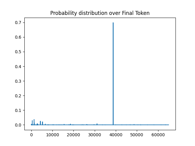
We can now print a ranked list of the highest probability next tokens:
# %% Now let's see what the highest probability tokens are.
# First we decode range(vocab_size) to get the string representation
# of each token in the vocabulary.
vocab_size = tokenizer.vocab_size
vocab = [tokenizer.decode([i]) for i in range(vocab_size)]

# sorted_idx will contain the indices that yield the sorted probabilities
# in descending order.
sorted_idx = np.argsort(next_token_probs)[::-1]

# Print out the top 10 tokens and their probabilities
for i in range(10):
    print(vocab[sorted_idx[i]], "\t\t",probs[-1,sorted_idx[i]], "\t\t", sorted_idx[i])
Paris       0.6987319       38765
par         0.03665255      1346
The         0.029361937     487
La          0.02517883      4317
Par         0.020812064     5336
the         0.014450773     1410
la          0.008413297     2854
France      0.0075454805    31126
PAR         0.005467169     18562
 Paris      0.00530823      6671
Looks like the model predicted the correct answer (Paris) with 69% probability!