Behold, a line attractor.
Will random linear systems pass the “line attractor test”?
Runnable Colab Research Notebook

"Behold a man" -- Diogenes of Sinope, see Diogenes 6 for historical account
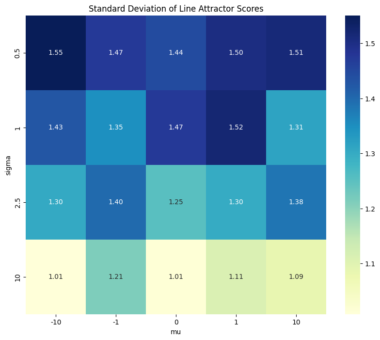
This code tests random \(d\) dimensional (default \(d=8\)) linear autonomous dynamical systems for the “Line Attractor Score” proposed in “An approximate line attractor in the hypothalamus encodes an aggressive state”.
I would like to know the expected rate of random systems \(\dot x = Ax\) passing the line attractor score cutoff of zero (or one, as sometimes implied).
From Nair A, Karigo T, Yang B, Ganguli S, Schnitzer MJ, Linderman SW, Anderson DJ, Kennedy A. An approximate line attractor in the hypothalamus encodes an aggressive state. Cell. 2023 Jan 5;186(1):178-193.e15. doi: 10.1016/j.cell.2022.11.027. PMID: 36608653; PMCID: PMC9990527.
Mathematical Description of the Experiment
1. Generating Random Linear Systems
For each trial in the experiment, we generate a random \(d \times d\) dynamics matrix \(A\) with entries drawn independently from a normal distribution with mean \(\mu\) and standard deviation \(\sigma\):
\[A_{ij} \sim N(\mu, \sigma^2)\]where \(i, j = 1, 2, \ldots, d\). This random matrix represents a linear system:
\[\frac{d\mathbf{x}}{dt} = A \mathbf{x}\]where \(\mathbf{x} \in \mathbb{R}^d\) is the state vector of the system.
2. Calculating Eigenvalues and Time Constants
For each matrix \(A\), we compute the eigenvalues \(\{\lambda_i\}_{i=1}^d\) by solving
\[\det(A - \lambda I) = 0\]where \(I\) is the \(d \times d\) identity matrix.
The time constant \(\tau_i\) associated with each eigenvalue \(\lambda_i\) is defined based on its magnitude:
\[\tau_i = \frac{1}{|\log(|\lambda_i|)|}\]Here, \(\|\lambda_i\|\) denotes the absolute value of the eigenvalue. This formula captures both real and complex eigenvalues by using the magnitude \(\|\lambda_i\|\), and it ensures all time constants are positive.
3. Sorting Time Constants
Once we have the set of time constants \(\{\tau_i\}_{i=1}^d\), we sort them in descending order:
\[\tau_{(1)} \geq \tau_{(2)} \geq \cdots \geq \tau_{(d)}\]where \(\tau_{(1)}\) is the largest time constant and \(\tau_{(2)}\) is the second largest.
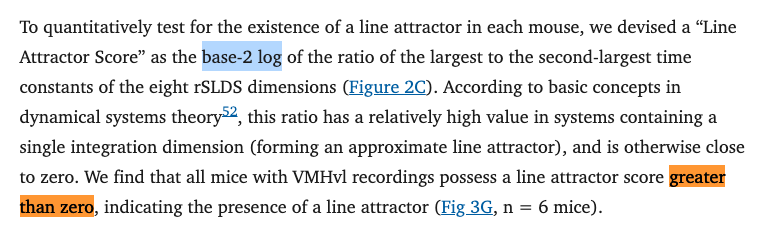
4. Line Attractor Score Calculation
The “Line Attractor Score” is calculated as the base-2 logarithm of the ratio between the largest and second-largest time constants:
\[\text{Line Attractor Score} = \log_2 \left( \frac{\tau_{(1)}}{\tau_{(2)}} \right)\]If this score is positive, it indicates that the largest time constant is significantly larger than the second largest, which, in theory, could suggest a line attractor.
Since \(\tau_{(1)} \geq \tau_{(2)}\) by construction, the argument to the logarithm must be \(\geq 1\). In my experience, \(\log(a) \geq 0\) if \(a \geq 1\) for any logarithm bases. Do email me if you discover this is not the case at abhargava (at) caltech (dot) edu.
5. Handling Complex Conjugates
If the top two time constants \(\tau_{(1)}\) and \(\tau_{(2)}\) are nearly identical, they may correspond to complex conjugate eigenvalues (e.g., \(\lambda = a \pm bi\)), which implies oscillatory dynamics rather than a true integrative line attractor. To address this:
- We set a threshold (e.g., \(10^{-10}\)) to determine if \(\tau_{(1)}\) and \(\tau_{(2)}\) are sufficiently close.
- If they are, we discard the complex conjugate and use the next unique time constant in the sorted list for \(\tau_{(2)}\), if available. If no distinct second time constant is found, we exclude this matrix from the Line Attractor Score calculation.
6. Simulation Procedure
We repeat the above steps over multiple trials, generating a new matrix \(A\) and calculating the Line Attractor Score for each trial. For each combination of parameters \((\mu, \sigma, d)\):
- Generate \(N\) random matrices \(A\).
- For each matrix, compute the Line Attractor Score.
- Calculate the proportion of matrices for which the Line Attractor Score is positive (i.e., \(\log_2 \left( \frac{\tau_{(1)}}{\tau_{(2)}} \right) > 0\)).
7. Reporting Results
The final result for each parameter set \((\mu, \sigma, d)\) is the estimated probability \(P(\text{Line Attractor Score} > 0)\) based on the proportion of trials that yielded a positive score:
\[P(\text{Line Attractor Score} > 0) = \frac{\text{Number of positive scores}}{N}\]These results are visualized in a heatmap that shows the likelihood of a positive Line Attractor Score across different values of \(\mu\) and \(\sigma\).
3 Figures
Histogram of line attractor scores for random matrices
Heatmap showing mean line attractor scores for various means/standard deviations for i.i.d. matrix entries in dynamics matrix A
Heatmap showing standard deviations of line attractor scores for various means/standard deviations
Figure 1g (Reference)
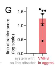
Figure 1g from the original paper showing their line attractor score distribution
Code
Check out the Runnable Colab Research Notebook to experiment with this code yourself. If you find any errors or have suggestions for improvements, please reach out to me at abhargava (at) caltech (dot) edu.
import numpy as np
import matplotlib.pyplot as plt
import seaborn as sns

# Background:
# In this analysis, we aim to test the likelihood that a randomly generated linear system,
# represented by a matrix A with entries drawn from a normal distribution N(mu, sigma),
# passes the "Line Attractor Score" test. The Line Attractor Score is based on the log-2
# ratio of the largest and second-largest time constants derived from the real parts of
# the eigenvalues of A. If the Line Attractor Score exceeds a certain threshold, the system
# is considered to have a line attractor-like structure, which in neuroscience may indicate
# persistent activity or integration along a particular direction.

# 1. Generate Random Matrix A
def generate_random_matrix(d, mu, sigma, do_sqrt_d=True):
    """
    Generates a d x d matrix with entries drawn independently from a normal distribution N(mu, sigma).

    Parameters:
        d (int): Dimension of the matrix.
        mu (float): Mean of the normal distribution.
        sigma (float): Standard deviation of the normal distribution.

    Returns:
        np.ndarray: A d x d random matrix.
    """
    if do_sqrt_d:
      return np.random.normal(mu, sigma/np.sqrt(d), (d, d))
    else:
      return np.random.normal(mu, sigma, (d, d))

# 2. Calculate the Line Attractor Score from eigenvalues
def calculate_line_attractor_score(matrix, use_imaginary_eigenvals=True, eliminate_complex_conjugates=True):
    """
    Calculates the Line Attractor Score (log2 ratio) for the given matrix based on its eigenvalues.
    Specifically, this is the log2 of the ratio of the largest to the second-largest time constants,
    where the time constants are computed from the real parts of the eigenvalues.

    Parameters:
        matrix (np.ndarray): A d x d square matrix representing the system dynamics.

    Returns:
        float or None: The Line Attractor Score if computable, otherwise None.

    Raises:
        TypeError: If the input is not a NumPy array.
        ValueError: If the input is not a square matrix.
    """

    # -------------------------
    # Input Validation
    # -------------------------

    # Check if the input is a NumPy array
    if not isinstance(matrix, np.ndarray):
        raise TypeError("Input must be a NumPy array representing a square matrix.")

    # Check if the matrix is square
    if matrix.ndim != 2 or matrix.shape[0] != matrix.shape[1]:
        raise ValueError(
            f"Input matrix must be square. Received shape {matrix.shape}."
        )

    # -------------------------
    # Eigenvalue Computation
    # -------------------------

    # Compute the eigenvalues of the matrix
    eigenvalues = np.linalg.eigvals(matrix)
    # Debug: print(f"Eigenvalues: {eigenvalues}")

    # Extract the real parts of the eigenvalues(?)
    # TODO: Ask to see if we should use the imaginary parts too -- the
    # "Dynamical system models of neural data" says \tau_i = |1/(log(|\lambda_a|))|
    # which is odd because usually time constants only deal with the real component.
    if use_imaginary_eigenvals:
        real_parts = np.abs(eigenvalues) # use the imaginary parts even though its weird
    else:
        real_parts = np.real(eigenvalues) # use the real parts like you normally do with time constants


    # Debug: print(f"Real parts of eigenvalues: {real_parts}")

    # -------------------------
    # Time Constants Calculation
    # -------------------------

    # Filter out eigenvalues with zero real parts to avoid division by zero
    # Time constants are computed as τ_i = -1 / Re(λ_i)
    # Only consider eigenvalues with non-zero real parts
    nonzero_real_parts = real_parts[np.nonzero(real_parts)]


    # Check if there are at least two eigenvalues with non-zero real parts
    if nonzero_real_parts.size < 2:
        # Not enough information to compute the Line Attractor Score
        assert False
        return None


    # Compute time constants: \tau_i = |1/(log(|\lambda_i|))|
    time_constants = np.abs(1.0 / np.abs(np.log(np.abs(nonzero_real_parts))))
    # Debug: print(f"Time constants: {time_constants}")

    # Take absolute values to handle cases where real parts are negative
    time_constants = np.abs(time_constants)
    # Debug:


    # -------------------------
    # Line Attractor Score Calculation
    # -------------------------

    # Sort the time constants in descending order (largest to smallest)
    sorted_time_constants = np.sort(time_constants)[::-1]

    # print(f"Time constants: {sorted_time_constants}")


    # Extract the largest and second-largest time constants
    if not eliminate_complex_conjugates:
        ## CRITICAL SECTION ##
        tau1 = sorted_time_constants[0]
        tau2 = sorted_time_constants[1]
        ## END CRITICAL SECTION ##
    else:
        ## CRITICAL SECTION ##
        # Extract the two largest time constants
        tau1 = sorted_time_constants[0]
        tau2 = sorted_time_constants[1]

        # If tau1 and tau2 are nearly identical, check if they come from complex conjugates
        if np.isclose(tau1, tau2):
            # Iterate through the sorted time constants to find the next unique time constant
            for time_constant in sorted_time_constants[2:]:
                if not np.isclose(time_constant, tau1, atol=1e-10):
                    tau2 = time_constant
                    break
            else:
                # If no unique second time constant is found, return None
                return None
        ## END CRITICAL SECTION ##


    # print unique versus sorted constnats
    # print(f"Unique time constants: {unique_time_constants}")
    # print(f"Sorted time constants: {sorted_time_constants}")
    # print(f"tau1: {tau1}, tau2: {tau2}")

    # Avoid division by zero or taking log of zero
    if tau2 == 0:
        # Cannot compute log2 of infinity or zero
        assert False
        return None

    # Compute the Line Attractor Score
    # Line Attractor Score = log2(tau1 / tau2)
    line_attractor_score = np.log2(tau1 / tau2)
    # Debug: print(f"Line Attractor Score: {line_attractor_score}")

    # if tau1==tau2:
        # print("COMPLEX CONJUGATE PAIR DETECTED, SCORE=", line_attractor_score)

    return line_attractor_score


# 3. Simulate the Line Attractor Scores for Random Systems
def simulate_line_attractor_scores(d, mu, sigma, num_samples=1000, use_imaginary_eigenvals=True, eliminate_complex_conjugates=True, do_sqrt_d=False):
    """
    Simulates a series of random matrices, computes the Line Attractor Score for each,
    and returns the distribution of these scores.

    Parameters:
        d (int): Dimension of the matrix.
        mu (float): Mean of the normal distribution for matrix entries.
        sigma (float): Standard deviation of the normal distribution for matrix entries.
        num_samples (int): Number of random matrices to generate.

    Returns:
        list: List of Line Attractor Scores for each generated matrix.
    """
    if use_imaginary_eigenvals:
      print("WARNING: Using |\lambda_a| rather than |Re(\lambda_a)| for time constant calculation.")
    else:
      print("WARNING: Using |Re(\lambda_a)| rather than |\lambda_a| for time constant calculation")
    scores = []
    for _ in range(num_samples):
        # Generate a random matrix with specified mean and variance
        matrix = generate_random_matrix(d, mu, sigma, do_sqrt_d=do_sqrt_d)
        # Calculate the Line Attractor Score for the generated matrix
        score = calculate_line_attractor_score(matrix, use_imaginary_eigenvals=use_imaginary_eigenvals, eliminate_complex_conjugates=eliminate_complex_conjugates)
        if score is not None:
            scores.append(score)  # Append only if score is valid (not None)
    return scores

# 4. Plot the Distribution of Line Attractor Scores
def plot_line_attractor_score_distribution(scores, mu, sigma, d):
    """
    Plots the distribution of Line Attractor Scores for a given set of simulation parameters.

    Parameters:
        scores (list): List of Line Attractor Scores from simulated matrices.
        mu (float): Mean of the normal distribution for matrix entries.
        sigma (float): Standard deviation of the normal distribution for matrix entries.
        d (int): Dimension of the matrix.
    """
    sns.histplot(scores, kde=True, bins=30, color='blue')
    plt.title(f"Line Attractor Score Distribution for A ~ N({mu}, {sigma}), d={d}")
    plt.xlabel("Line Attractor Score (log2 ratio)")
    plt.ylabel("Frequency")
    plt.show()

# 5. Calculate the Likelihood of Passing the Line Attractor Score Threshold
def likelihood_above_threshold(scores, threshold=0):
    """
    Calculates and prints the likelihood of the Line Attractor Score exceeding a specified threshold.

    Parameters:
        scores (list): List of Line Attractor Scores from simulated matrices.
        threshold (float): The threshold above which we consider the score to "pass" the test.
                           Default is 0, as per the paper.

    Returns:
        float: Likelihood (percentage) of the scores exceeding the threshold.
    """
    # Count the number of scores that exceed the threshold (default 0)
    above_threshold = [score for score in scores if score > threshold]
    # Calculate the proportion of scores above the threshold
    likelihood = len(above_threshold) / len(scores) if scores else 0
    # Print the likelihood as a percentage
    print(f"Likelihood of Line Attractor Score > {threshold}: {likelihood * 100:.2f}%")
    return likelihood


# 6. Run Comprehensive Simulations and Analyze Likelihoods

```python
def run_comprehensive_simulation(d_values, mu_values, sigma_values, num_samples=1000, threshold=1.0, do_plot=True, use_imaginary_eigenvals=True, eliminate_complex_conjugates=True, do_sqrt_d=False):
    """
    Runs simulations over a range of parameter values, plotting the distribution of Line Attractor Scores
    and calculating the likelihood of scores exceeding the threshold for each set of parameters.

    Parameters:
        d_values (list): List of dimensions to simulate.
        mu_values (list): List of mean values for matrix entries.
        sigma_values (list): List of standard deviation values for matrix entries.
        num_samples (int): Number of random matrices to simulate for each parameter set.
        threshold (float): The threshold for passing the Line Attractor Score test.
    """
    results_dicts = []
    for d in d_values:
        for mu in mu_values:
            for sigma in sigma_values:
                # Simulate the scores for the current set of parameters
                scores = simulate_line_attractor_scores(d, mu, sigma, num_samples, use_imaginary_eigenvals=use_imaginary_eigenvals, eliminate_complex_conjugates=eliminate_complex_conjugates, do_sqrt_d=do_sqrt_d)

                # Plot the distribution of scores
                if scores:
                    if do_plot:
                        plot_line_attractor_score_distribution(scores, mu, sigma, d)
                    # print params
                    print(f"d = {d}, mu = {mu}, sigma = {sigma}")

                    # Calculate and print the likelihood of passing the threshold
                    lik_above_thresh = likelihood_above_threshold(scores, threshold)

                else:
                  assert False

                result_dict = {
                    "d": d,
                    "mu": mu,
                    "sigma": sigma,
                    "num_samples": num_samples,
                    "threshold": threshold,
                    "likelihood": lik_above_thresh,
                    "scores": scores
                }
                results_dicts.append(result_dict)
    return results_dicts


# Invocation Code: Define ranges for matrix dimension, mean, and variance to explore
# For example, we could test dimensions of 3, means of 0 and 1, and standard deviations of 0.5 and 2
d_values = [8]                 # Dimension of the matrix, often small in neuroscience models
mu_values = [-10, -1, 0, 1, 10]             # Means for normal distribution of matrix entries
sigma_values = [0.5, 1, 2.5, 10]        # Standard deviations for normal distribution of matrix entries
num_samples = 1000             # Number of random matrices to generate for each parameter set
threshold = 0.0                # Threshold for Line Attractor Score test
do_plot=True                   # plot histograms of line attractor scores for each distribution of a_ij~N(mu, sigma)
use_imaginary_eigenvals = True
eliminate_complex_conjugates = True # True -> if the largest time constant's eigenvalue is complex, we don't just compare it to itself leading to log(tau_max/tau_max) = log(1) = 0 every time
do_sqrt_d = False # divide sigma by sqrt(d=8) to normalize a_ij~N(mu, sigma/sqrt(d))

# Run the comprehensive simulation
results_dicts = run_comprehensive_simulation(d_values, mu_values, sigma_values, num_samples, threshold,
                                             do_plot=do_plot,
                                             use_imaginary_eigenvals=use_imaginary_eigenvals,
                                             eliminate_complex_conjugates=eliminate_complex_conjugates,
                                             do_sqrt_d=do_sqrt_d)
def plot_likelihood_heatmaps(results_dicts, x_param='mu', y_param='sigma', z_param='likelihood', d_param='d', cmap='viridis', threshold=0.0):
    """
    Plots heatmaps of likelihood scores from a list of results dictionaries.
    Each heatmap corresponds to a specific value of 'd' (dimension), and shows the likelihood scores
    across combinations of 'mu' and 'sigma'.

    Parameters:
        results_dicts (list): A list of dictionaries containing simulation results.
                              Each dictionary should have keys including 'd', 'mu', 'sigma', and the score key.
        x_param (str): The name of the parameter to plot on the x-axis (default 'mu').
        y_param (str): The name of the parameter to plot on the y-axis (default 'sigma').
        z_param (str): The name of the parameter to use for the heatmap values (default 'likelihood').
        d_param (str): The name of the dimension parameter in the results dictionaries (default 'd').
        cmap (str): The colormap to use for the heatmap (default 'viridis').

    Returns:
        None: Displays the heatmap plots.
    """

    # -------------------------
    # Input Validation
    # -------------------------

    # Check if 'results_dicts' is a list
    if not isinstance(results_dicts, list):
        raise TypeError("The 'results_dicts' parameter must be a list of dictionaries.")

    # Check if the list is not empty
    if not results_dicts:
        raise ValueError("The 'results_dicts' list is empty.")

    # Extract the keys from the first dictionary to validate parameter names
    sample_dict = results_dicts[0]
    required_keys = {x_param, y_param, z_param, d_param}

    # Check if all required keys are present
    if not required_keys.issubset(sample_dict.keys()):
        missing_keys = required_keys - sample_dict.keys()
        raise KeyError(f"The following required keys are missing in the results dictionaries: {missing_keys}")

    # -------------------------
    # Data Preparation
    # -------------------------

    # Extract all unique 'd' values
    d_values = sorted(set(result[d_param] for result in results_dicts))

    # For each 'd', prepare data and plot heatmap
    for d in d_values:
        # Filter results for the current dimension 'd'
        filtered_results = [res for res in results_dicts if res[d_param] == d]

        # Extract unique 'mu' and 'sigma' values
        x_values = sorted(set(res[x_param] for res in filtered_results))
        y_values = sorted(set(res[y_param] for res in filtered_results))

        # Debug: print(f"d = {d}, x_values = {x_values}, y_values = {y_values}")

        # Initialize a 2D array to hold the likelihood scores
        # The shape is (number of y_values, number of x_values)
        heatmap_data = np.full((len(y_values), len(x_values)), np.nan)

        # Create mappings from parameter values to indices
        x_to_index = {value: idx for idx, value in enumerate(x_values)}
        y_to_index = {value: idx for idx, value in enumerate(y_values)}

        # Populate the heatmap data matrix
        for res in filtered_results:
            x_val = res[x_param]
            y_val = res[y_param]
            z_val = res[z_param]

            # Get indices
            x_idx = x_to_index[x_val]
            y_idx = y_to_index[y_val]

            # Assign the z value to the heatmap data
            heatmap_data[y_idx, x_idx] = z_val

        # -------------------------
        # Plotting the Heatmap
        # -------------------------

        # Set up the matplotlib figure
        plt.figure(figsize=(10, 8))

        # Use seaborn heatmap to plot the data
        sns.heatmap(
            heatmap_data,
            xticklabels=x_values,
            yticklabels=y_values,
            cmap=cmap,
            annot=True,
            fmt=".2f",
            cbar_kws={'label': z_param.replace('_', ' ').title()},
            # Handle NaN values appropriately
            mask=np.isnan(heatmap_data)
        )

        # Set the axis labels and title
        plt.xlabel(x_param)
        plt.ylabel(y_param)
        # plt.title(f'Heatmap of {z_param.replace("_", " ").title()} for {d_param} = {d}')
        plt.title(f'Heatmap of likelihood of passing log2(time const ratio) > {threshold}')

        # Optionally invert the y-axis to have lower y values at the bottom
        plt.gca().invert_yaxis()

        # Improve layout
        plt.tight_layout()

        # Display the plot
        plt.show()

# Call plot likelihood score function
plot_likelihood_heatmaps(results_dicts, threshold=threshold)

print(f"Use imaginary eigenvals={use_imaginary_eigenvals}\nEliminate complex conjugates={eliminate_complex_conjugates}\nThreshold for log_2(tau_max/tau_[max-1]): {threshold}\nDo square root d: {do_sqrt_d}")
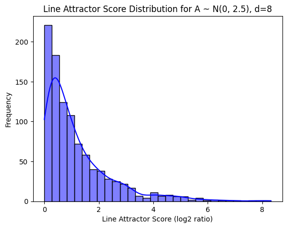
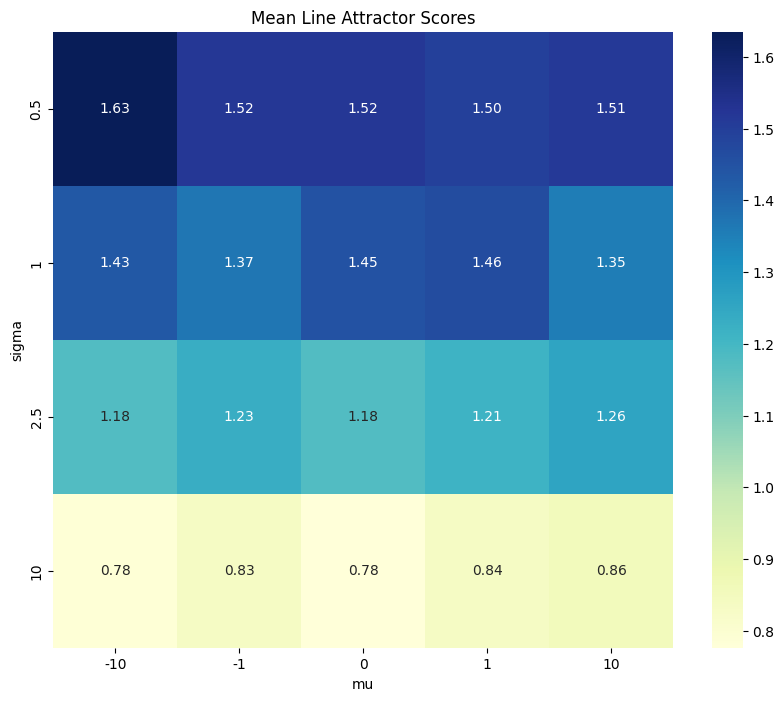
def plot_mean_std_heatmap(results_dicts, mu_values, sigma_values, d_values):
    """
    Creates a heatmap of the mean Line Attractor Scores and standard deviation for each combination of mu and sigma.

    Parameters:
        results_dicts (list): List of dictionaries containing the results for each combination of parameters.
                              Each dictionary should have "mu", "sigma", and "scores" (list of scores).
        mu_values (list): List of mean values for matrix entries.
        sigma_values (list): List of standard deviation values for matrix entries.
        d_values (list): List of dimensions tested (the heatmap will aggregate across these if more than one).
    """
    # Prepare matrices to store the mean and standard deviation for each (mu, sigma) combination
    mean_scores = np.zeros((len(sigma_values), len(mu_values)))
    std_scores = np.zeros((len(sigma_values), len(mu_values)))

    # Populate the matrices with the mean and standard deviation of scores
    for result in results_dicts:
        mu_index = mu_values.index(result["mu"])
        sigma_index = sigma_values.index(result["sigma"])

        # Calculate mean and standard deviation of scores for the current (mu, sigma) combination
        scores = result["scores"]
        mean_scores[sigma_index, mu_index] = np.mean(scores)
        std_scores[sigma_index, mu_index] = np.std(scores)

    # Plot heatmap of mean scores
    plt.figure(figsize=(10, 8))
    ax = sns.heatmap(mean_scores, annot=True, fmt=".2f", cmap="YlGnBu", xticklabels=mu_values, yticklabels=sigma_values)
    ax.set_title("Mean Line Attractor Scores")
    ax.set_xlabel("mu")
    ax.set_ylabel("sigma")
    plt.show()

    # Plot heatmap of standard deviation of scores
    plt.figure(figsize=(10, 8))
    ax = sns.heatmap(std_scores, annot=True, fmt=".2f", cmap="YlGnBu", xticklabels=mu_values, yticklabels=sigma_values)
    ax.set_title("Standard Deviation of Line Attractor Scores")
    ax.set_xlabel("mu")
    ax.set_ylabel("sigma")
    plt.show()

# run code
plot_mean_std_heatmap(results_dicts, mu_values, sigma_values, d_values)
Even with threshold 1, most random systems pass line attractor test
# Invocation Code: Define ranges for matrix dimension, mean, and variance to explore
# For example, we could test dimensions of 3, means of 0 and 1, and standard deviations of 0.5 and 2
d_values = [8]                 # Dimension of the matrix, often small in neuroscience models
mu_values = [-10, -1, 0, 1, 10]             # Means for normal distribution of matrix entries
sigma_values = [0.5, 1, 2.5, 10]        # Standard deviations for normal distribution of matrix entries
num_samples = 1000             # Number of random matrices to generate for each parameter set
threshold = 1.0                # Threshold for Line Attractor Score test
do_plot=False                   # plot histograms of line attractor scores for each distribution of a_ij~N(mu, sigma)
use_imaginary_eigenvals = True
eliminate_complex_conjugates = True # True -> if the largest time constant's eigenvalue is complex, we don't just compare it to itself leading to log(tau_max/tau_max) = log(1) = 0 every time
do_sqrt_d = False # divide sigma by sqrt(d=8) to normalize a_ij~N(mu, sigma/sqrt(d))

# Run the comprehensive simulation
results_dicts = run_comprehensive_simulation(d_values, mu_values, sigma_values, num_samples, threshold,
                                             do_plot=do_plot,
                                             use_imaginary_eigenvals=use_imaginary_eigenvals,
                                             eliminate_complex_conjugates=eliminate_complex_conjugates,
                                             do_sqrt_d=do_sqrt_d)
plot_likelihood_heatmaps(results_dicts, threshold=threshold)
def plot_likelihood_heatmaps(results_dicts, threshold=0.0):
    """
    Plots heatmaps of likelihood scores from a list of results dictionaries.
    Each heatmap corresponds to a specific value of 'd' (dimension), and shows the likelihood scores
    across combinations of 'mu' and 'sigma'.

    Parameters:
        results_dicts (list): A list of dictionaries containing simulation results.
                              Each dictionary should have keys including 'd', 'mu', 'sigma', and the score key.
        threshold (float): The threshold above which we consider the score to "pass" the test.
    """

    # -------------------------
    # Input Validation
    # -------------------------

    # Check if 'results_dicts' is a list
    if not isinstance(results_dicts, list):
        raise TypeError("The 'results_dicts' parameter must be a list of dictionaries.")

    # Check if the list is not empty
    if not results_dicts:
        raise ValueError("The 'results_dicts' list is empty.")

    # Extract the keys from the first dictionary to validate parameter names
    sample_dict = results_dicts[0]
    required_keys = {'d', 'mu', 'sigma', 'likelihood'}

    # Check if all required keys are present
    if not required_keys.issubset(sample_dict.keys()):
        missing_keys = required_keys - sample_dict.keys()
        raise KeyError(f"The following required keys are missing in the results dictionaries: {missing_keys}")

    # -------------------------
    # Data Preparation
    # -------------------------

    # Extract all unique 'd' values
    d_values = sorted(set(result['d'] for result in results_dicts))

    # For each 'd', prepare data and plot heatmap
    for d in d_values:
        # Filter results for the current dimension 'd'
        filtered_results = [res for res in results_dicts if res['d'] == d]

        # Extract unique 'mu' and 'sigma' values
        x_values = sorted(set(res['mu'] for res in filtered_results))
        y_values = sorted(set(res['sigma'] for res in filtered_results))

        # Debug: print(f"d = {d}, x_values = {x_values}, y_values = {y_values}")

        # Initialize a 2D array to hold the likelihood scores
        # The shape is (number of y_values, number of x_values)
        heatmap_data = np.full((len(y_values), len(x_values)), np.nan)

        # Create mappings from parameter values to indices
        x_to_index = {value: idx for idx, value in enumerate(x_values)}
        y_to_index = {value: idx for idx, value in enumerate(y_values)}

        # Populate the heatmap data matrix
        for res in filtered_results:
            x_val = res['mu']
            y_val = res['sigma']
            z_val = res['likelihood']

            # Get indices
            x_idx = x_to_index[x_val]
            y_idx = y_to_index[y_val]

            # Assign the z value to the heatmap data
            heatmap_data[y_idx, x_idx] = z_val

        # -------------------------
        # Plotting the Heatmap
        # -------------------------

        # Set up the matplotlib figure
        plt.figure(figsize=(10, 8))

        # Use seaborn heatmap to plot the data
        sns.heatmap(
            heatmap_data,
            xticklabels=x_values,
            yticklabels=y_values,
            cmap='viridis',
            annot=True,
            fmt=".2f",
            cbar_kws={'label': 'Likelihood of passing log2(time const ratio) > 0'},
            # Handle NaN values appropriately
            mask=np.isnan(heatmap_data)
        )

        # Set the axis labels and title
        plt.xlabel('mu')
        plt.ylabel('sigma')
        plt.title(f'Heatmap of likelihood of passing log2(time const ratio) > {threshold}')

        # Optionally invert the y-axis to have lower y values at the bottom
        plt.gca().invert_yaxis()

        # Improve layout
        plt.tight_layout()

        # Display the plot
        plt.show()

# Call plot likelihood score function
plot_likelihood_heatmaps(results_dicts, threshold=threshold)

print(f"Use imaginary eigenvals={use_imaginary_eigenvals}\nEliminate complex conjugates={eliminate_complex_conjugates}\nThreshold for log_2(tau_max/tau_[max-1]): {threshold}\nDo square root d: {do_sqrt_d}")
def plot_mean_std_heatmap(results_dicts, mu_values, sigma_values, d_values):
    """
    Creates a heatmap of the mean Line Attractor Scores and standard deviation for each combination of mu and sigma.

    Parameters:
        results_dicts (list): List of dictionaries containing the results for each combination of parameters.
                              Each dictionary should have "mu", "sigma", and "scores" (list of scores).
        mu_values (list): List of mean values for matrix entries.
        sigma_values (list): List of standard deviation values for matrix entries.
        d_values (list): List of dimensions tested (the heatmap will aggregate across these if more than one).
    """
    # Prepare matrices to store the mean and standard deviation for each (mu, sigma) combination
    mean_scores = np.zeros((len(sigma_values), len(mu_values)))
    std_scores = np.zeros((len(sigma_values), len(mu_values)))

    # Populate the matrices with the mean and standard deviation of scores
    for result in results_dicts:
        mu_index = mu_values.index(result["mu"])
        sigma_index = sigma_values.index(result["sigma"])

        # Calculate mean and standard deviation of scores for the current (mu, sigma) combination
        scores = result["scores"]
        mean_scores[sigma_index, mu_index] = np.mean(scores)
        std_scores[sigma_index, mu_index] = np.std(scores)

    # Plot heatmap of mean scores
    plt.figure(figsize=(10, 8))
    ax = sns.heatmap(mean_scores, annot=True, fmt=".2f", cmap="YlGnBu", xticklabels=mu_values, yticklabels=sigma_values)
    ax.set_title("Mean Line Attractor Scores")
    ax.set_xlabel("mu")
    ax.set_ylabel("sigma")
    plt.show()

    # Plot heatmap of standard deviation of scores
    plt.figure(figsize=(10, 8))
    ax = sns.heatmap(std_scores, annot=True, fmt=".2f", cmap="YlGnBu", xticklabels=mu_values, yticklabels=sigma_values)
    ax.set_title("Standard Deviation of Line Attractor Scores")
    ax.set_xlabel("mu")
    ax.set_ylabel("sigma")
    plt.show()

# run code
plot_mean_std_heatmap(results_dicts, mu_values, sigma_values, d_values)
Even with threshold 1, most random systems pass line attractor test
# Invocation Code: Define ranges for matrix dimension, mean, and variance to explore
# For example, we could test dimensions of 3, means of 0 and 1, and standard deviations of 0.5 and 2
d_values = [8]                 # Dimension of the matrix, often small in neuroscience models
mu_values = [-10, -1, 0, 1, 10]             # Means for normal distribution of matrix entries
sigma_values = [0.5, 1, 2.5, 10]        # Standard deviations for normal distribution of matrix entries
num_samples = 1000             # Number of random matrices to generate for each parameter set
threshold = 1.0                # Threshold for Line Attractor Score test
do_plot=False                   # plot histograms of line attractor scores for each distribution of a_ij~N(mu, sigma)
use_imaginary_eigenvals = True
eliminate_complex_conjugates = True # True -> if the largest time constant's eigenvalue is complex, we don't just compare it to itself leading to log(tau_max/tau_max) = log(1) = 0 every time
do_sqrt_d = False # divide sigma by sqrt(d=8) to normalize a_ij~N(mu, sigma/sqrt(d))

# Run the comprehensive simulation
results_dicts = run_comprehensive_simulation(d_values, mu_values, sigma_values, num_samples, threshold,
                                             do_plot=do_plot,
                                             use_imaginary_eigenvals=use_imaginary_eigenvals,
                                             eliminate_complex_conjugates=eliminate_complex_conjugates,
                                             do_sqrt_d=do_sqrt_d)
plot_likelihood_heatmaps(results_dicts, threshold=threshold)